Previous
Forecasting Crop Prices in Ethiopia
29 June 2018 on posts
My objective here was to see how well I could predict historical crop prices in Ethiopia using solely weather and climate information. I chose to focus my analysis in Amhara, located in the Ethiopian highlands.
The main questions I was trying to answer here were:
-
How well can prices be predicted using solely climate and weather data?
-
How does this compare to models that include a lag term (i.e. information about previous prices)?
If models using solely weather and climate are on par with those using a lag term, this gives evidence that there is a relationship between climate and prices that is independent of previous price conditions.
Data
Crop prices
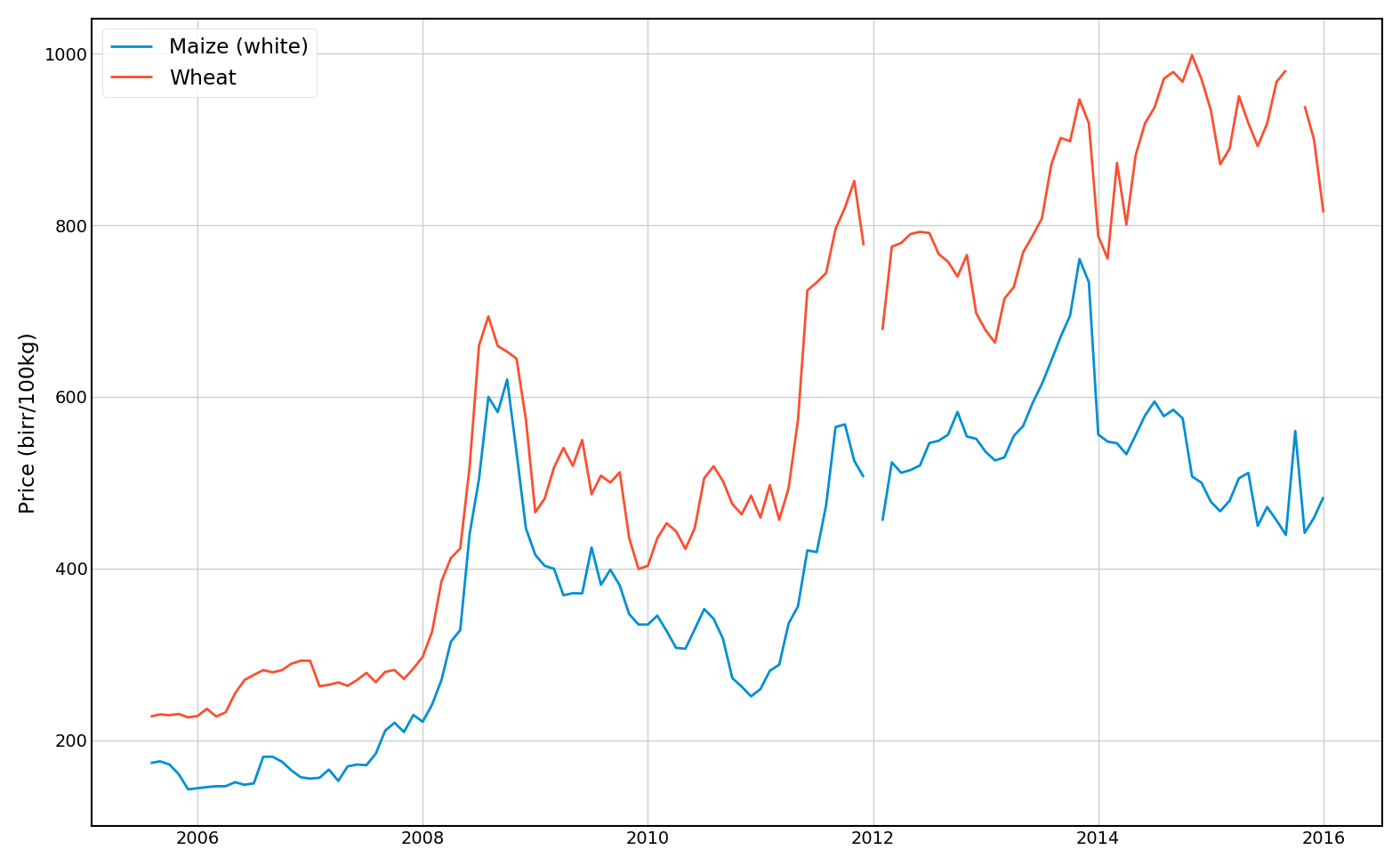
I sourced monthly crop prices for Maize and Wheat from the World Food Program’s online crop prices database.. This contains prices sourced from a variety of different markets within Amhara, which I simply averaged in each month. The final dataset contains monthly prices (with some missing values) from 2005 to 2015.
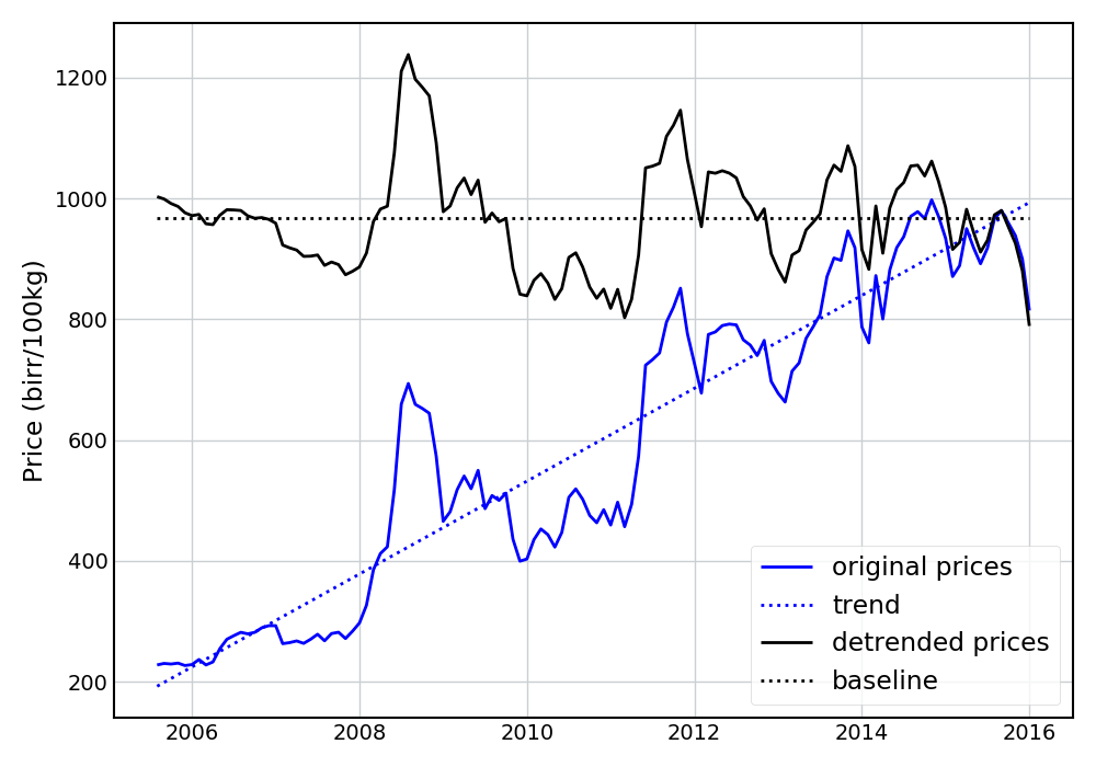
I then de-trended the prices (using a linear trend) and set them to a 2015 baseline value. The following figure shows the resulting prices for Wheat.
Climate
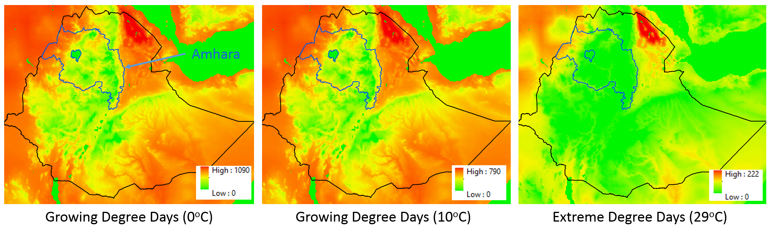
I began with historical daily gridded estimates (0.05 degree resolution) of rainfall (from CHIRPS) and maximum and minimum temperatures (from GDAS). From these, I developed monthly estimates of growing degree days (GDDs) (using base temperatures of 0 and 10 degrees Celsius for Wheat and Maize respectively) and extreme degree days (EDDs) (using a temperature of 29 degrees Celsius). The following figure shows these data over Ethiopia for April 2000. I then “regionalized” these rasters, simply taking the average value over Amhara for each month.
Dataset
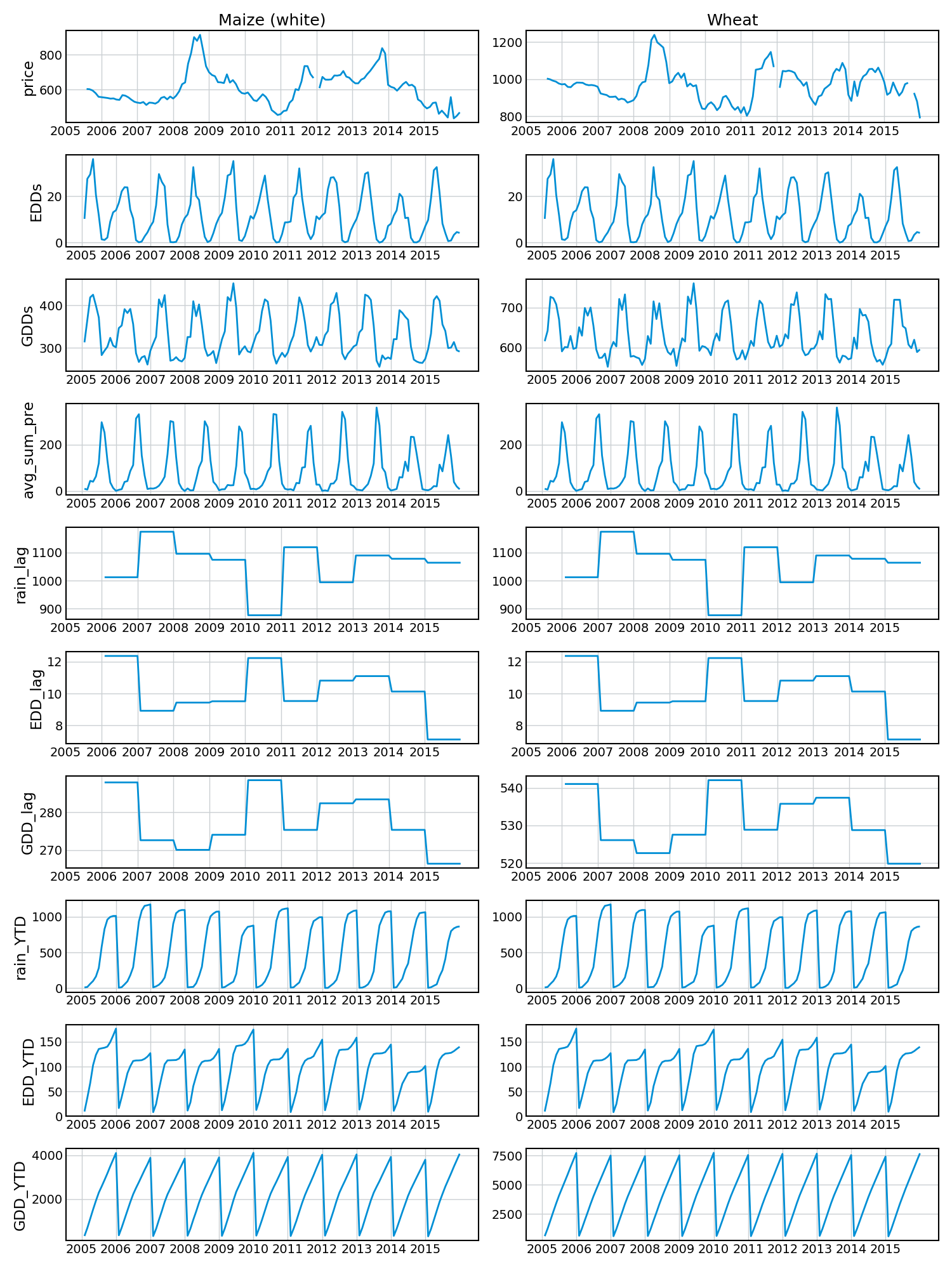
Using these data I created a dataset for each crop with the following covariates:
| Column | Description |
|---|---|
| year | Year |
| month | Month |
| price | Price in birr / 100kg |
| EDDs | Regionalized average EDDs for this month |
| GDDs | Regionalized average GDDs for this month |
| avg_sum_pre | Regionalized average total precipitation for this month |
| rain_lag | Regionalized average total precipitation from the previous year |
| EDD_lag | Regionalized average total EDDs from the previous year |
| GDD_lag | Regionalized average total GDDs from the previous year |
| rain_YTD | Total year-to-date sum of rainfall |
| EDD_YTD | Total year-to-date sum of EDDs |
| GDD_YTD | Total year-to-date sum of GDDs |
The following figure shows these covariates over time for the two crops.
Modeling
Simple linear models
The first model I fit was a simple linear regression using all covariates. I trained the model to the entire dataset. Note that this isn’t ideal best-practice, as I am evaluating my predictions based on data that the model has already seen, but it’s a first attempt. The following figure shows the predicted vs. actual values using this linear model for Maize and then Wheat.
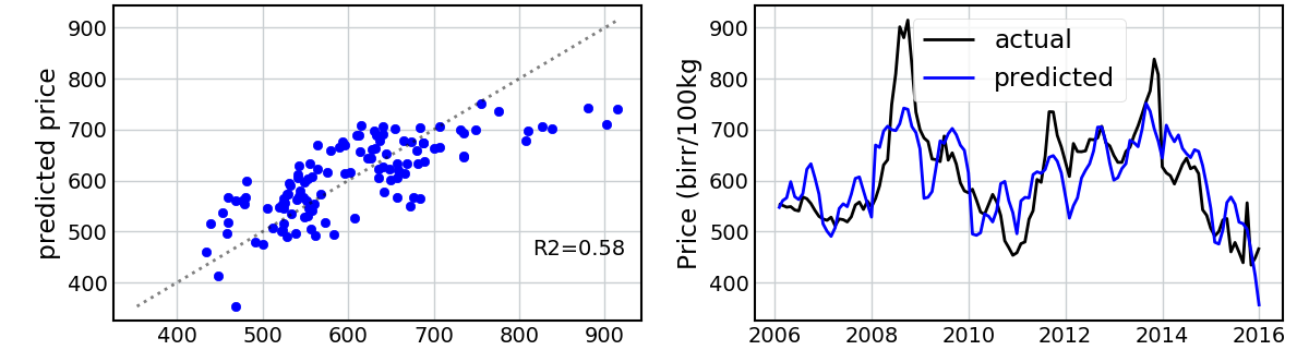
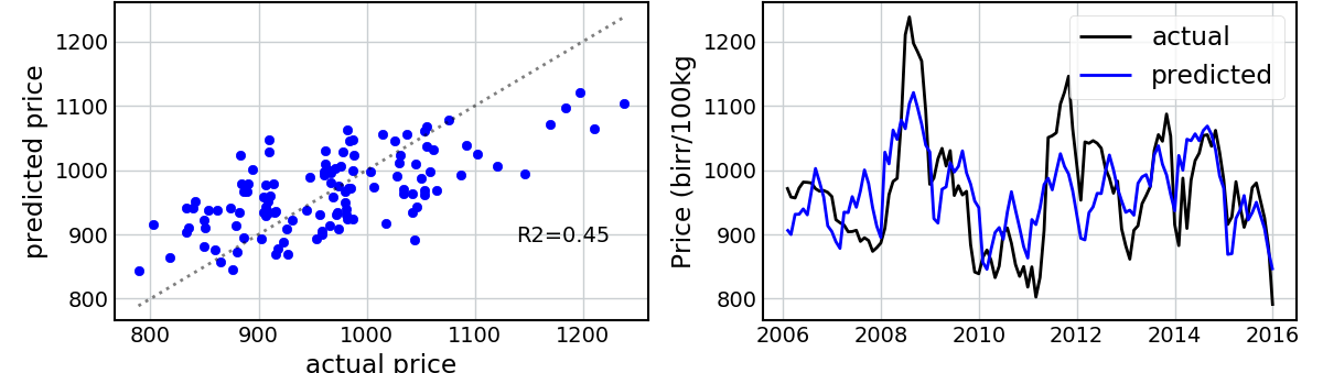
This is surprisingly good! I’m not able to capture the extreme values, but the model does a reasonable job of explaining the variance in the prices and capturing the peaks and troughs of the time series.
But am I considerably overestimating my predictive accuracy by using the entire dataset?
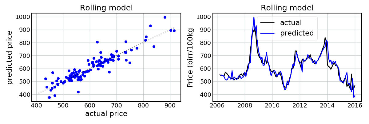
To get around this, I created a “rolling model”, in which I predicted each month’s price using only the data that had previously been observed. For example, to predict the dataset’s second month’s price I trained a model only on the information from the first month. Each month I added an additional month’s worth of data to the dataset.
How do we do?
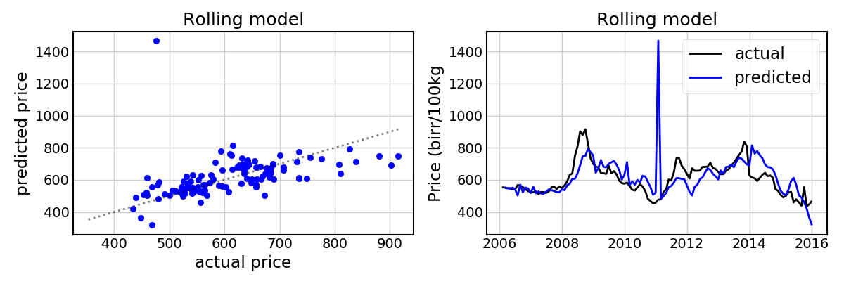
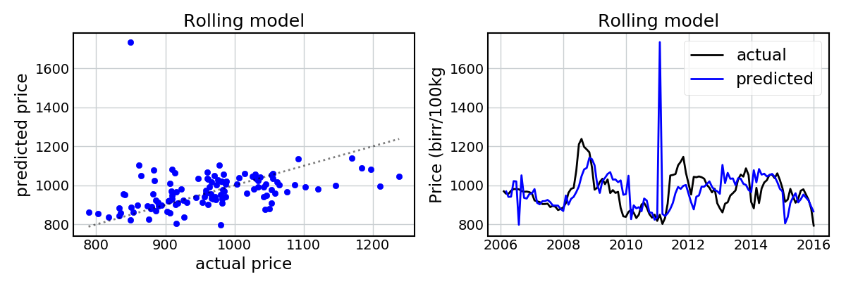
Still very well (apart from a spurious month in 2011, which I believe is a sign of the model’s sensitivity to the abnormally low rainfall and high temperatures in the previous year (refer to the figure showing the temporal evolution of the covariates) – but this is not entirely clear). Again, we’re able to capture the general trends in the data. The model does pretty badly at predicting Wheat prices in 2013 (i.e. it predicts a price increase, rather than a price decrease), and again the extreme values are not always predicted, but I’m still pretty impressed.
So, to give a preliminary answer to question #1 above, prices can be predicted reasonably accurately using solely climate information.
Adding a lag term
Say we’re trying to predict what the price will be next month (in July). We know what the price was now (in June), so why not utilize this information for our prediction? To assess this, I simply added an extra covariate representing the price from the previous month. The following figures show the predictions for Maize and Wheat using a “rolling” linear model with a lag term.
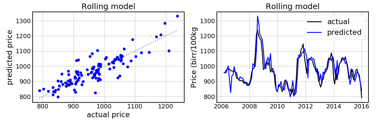
This has improved the model fit considerably! Given we know the previous price, we’re now able to capture the pits and peaks in the dataset with a high amount of accuracy.
This is not unexpected, and gives us a preliminary answer to question #2 above. It seems that the inclusion of the lag term does help improve the predictions considerably. But now let’s assess this quantitatively…
Testing out-of-sample accuracy (and variable selection)
An alternative way of evaluating model performance is to conduct a holdout analysis. Here, I trained a linear model on a random 80% of the data, and then tested it on the remaining 20%. I repeated this 50 times, giving a distribution of predictive accuracy.
I also added a backwards stepwise variable selection (using sklearn.feature_selection.RFE) to see how the predictive accuracy depends on the number of covariates that are included.
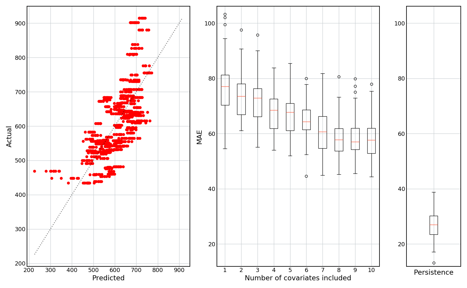
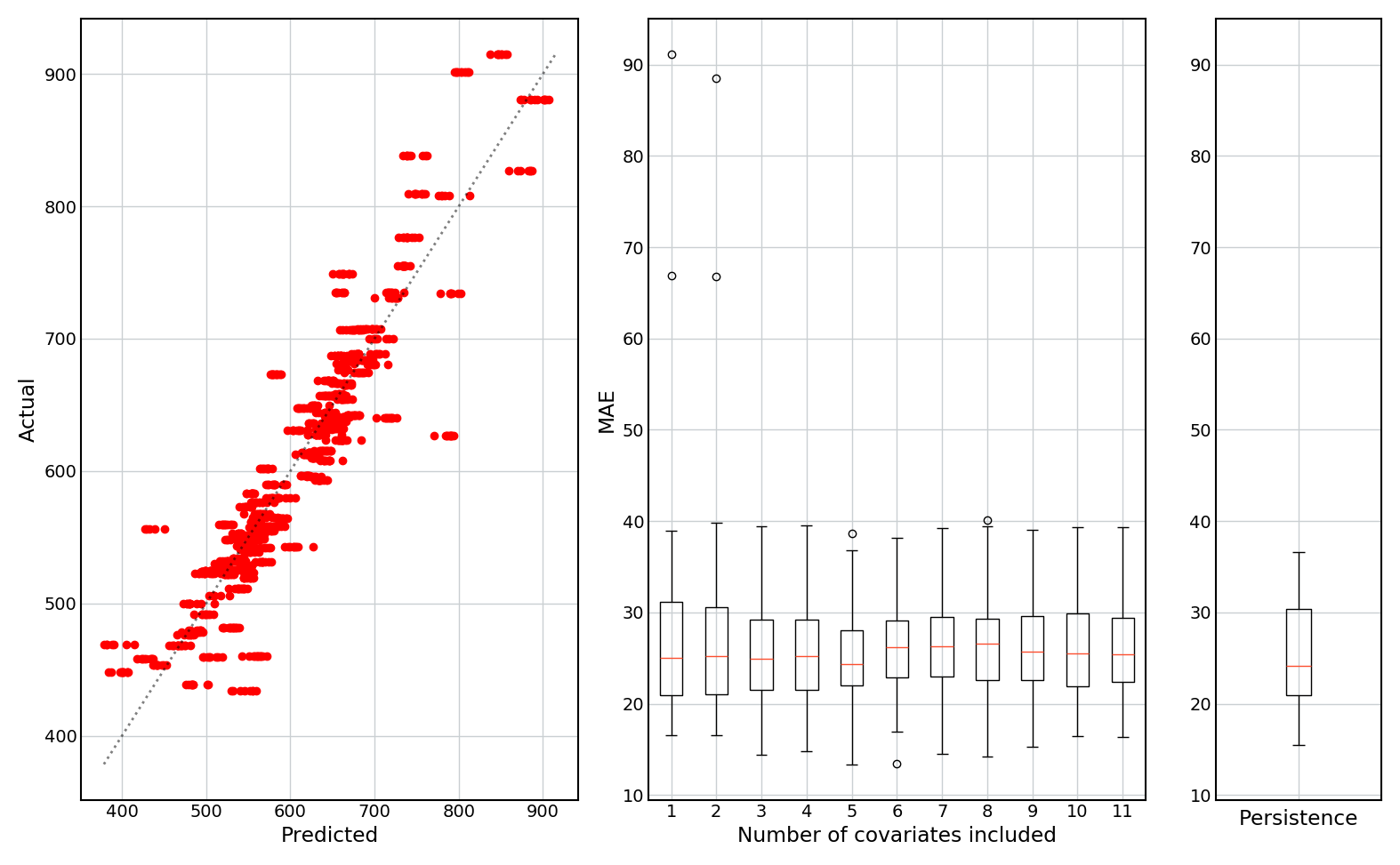
The following figures show: (1) predicted vs actual values (for all 50 holdouts); (2) boxplots of the mean absolute prediction error (MAE) as a function of the number of covariates included; and (3) a boxplot of the MAE of the persistence model (i.e. if the prediction is set equal to last month’s value).
Results are shown for models without and with a lag term (only the results for Maize are shown for brevity, but the results for Wheat are similar).
No lag term:
With lag term:
Some observations:
- The model with no lag term fails to predict the extreme values.
- Inclusion of the lag term significantly improves the predictive accuracy, and gives better predictions of extreme values.
- The lag term, when included, is (likely) by far the most important predictor of prices, as adding additional covariates does not noticeably improve the MAE.
- When no lag term is included, more covariates generally leads to better predictions.
- Without a lag term, none of the models ever do as well as the persistence model, and achieve MAEs that are approximately twice as high as the persistence model.
Based on this final point, I can conclude that I may have some pretty graphs so far, but the models are pretty useless at predicting month-ahead crop yields.
Based on this, I conclude that:
- Yes, crop prices can be predicted using solely climate and weather data. However, these models struggle at predicting extreme values.
- Including a lag term (or running a simple persistence model) gives predictions that are twice as accurate.
Variable importance
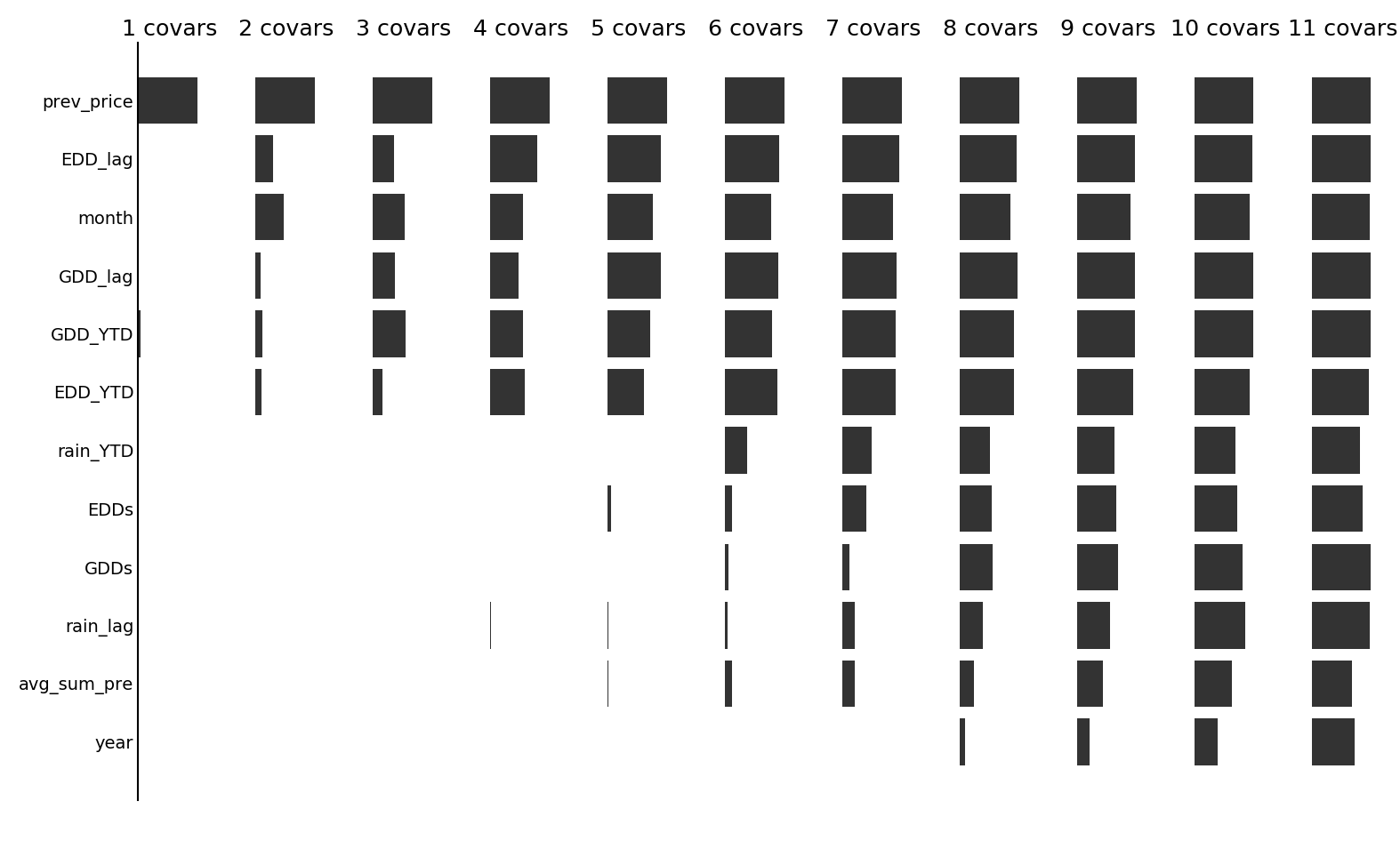
Which variables are the most useful for predicting prices? The following two figures show (for Maize), for each number of covariates in the stepwise selection algorithm, the frequency with which each covariate was selected.
With a lag term (prev_price):
Without a lag term:
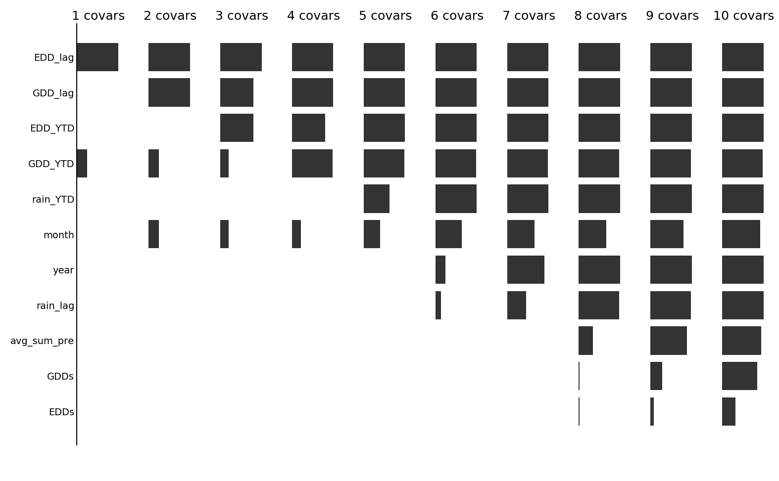
We see that, as expected, when the lag term is included, it is almost always retained as a variable. Following this, it generally seems that the temperature (EDD and GDD) variables are selected more often than the rainfall variables, suggesting that prices might be more closely related to temperature than rainfall.
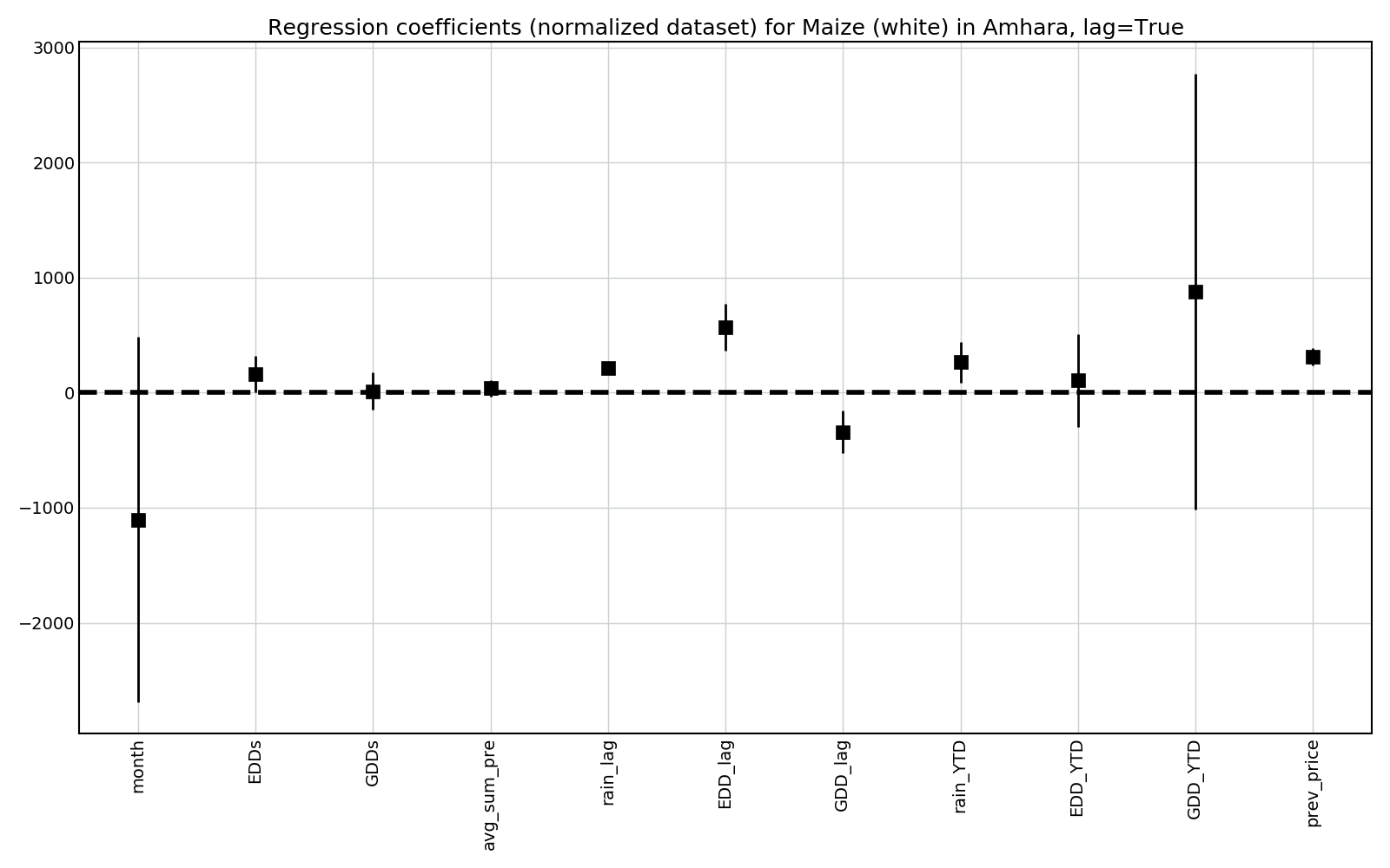
We can also look at the value of the regression parameters to see the direction with which each coefficient influences prices.
For this, all data was normalized (using sklearn.preprocessing.MinMaxScaler).
Some observations:
- EDDs (and lagged EDDs) has a positive coefficient, so more EDDs is associated with higher crop prices. This is intuitive, as EDDs can have detrimental effects on crop yields.
- The effect of both GDDs and EDDs in the previous year is more significant than both the current month’s value and the year-to-date sum. This is interesting, and offers hope that longer-range forecasts will be possible.
- More rain seems to lead to higher prices.
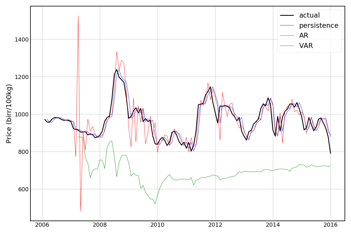
Autoregressive models
Adding a lag term is slightly in the spirit of an autoregressive (AR) model, which are specifically intended for time series analysis. I’ve never worked with these before, but decided to have a preliminary stab at building some.
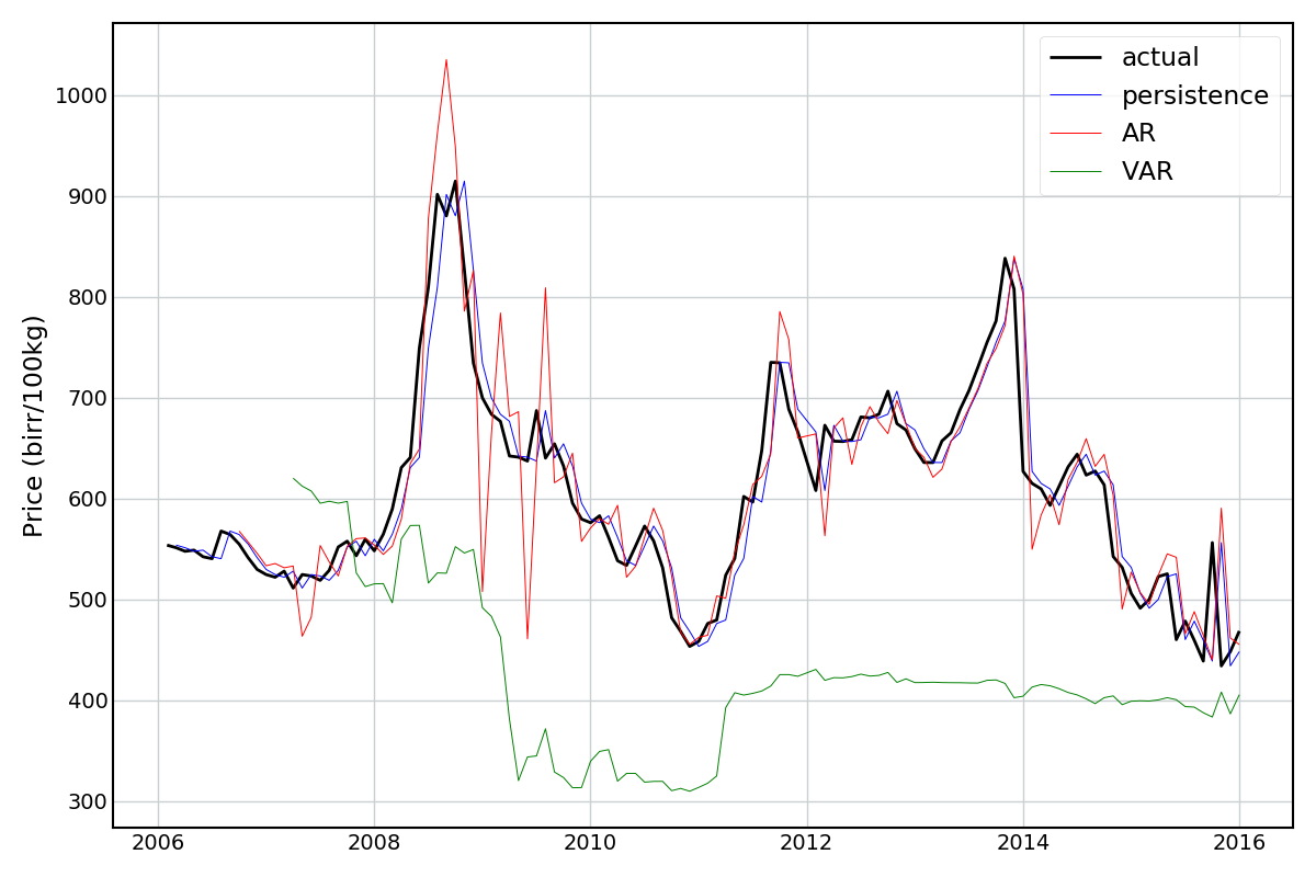
The “null” model here is what is called a persistence model, i.e. just predicting the value from the previous period. The AR model is a regression model that predicts/forecasts the price given the history of prices. If an AR model can’t do better than the persistence model, then there’s not much point. A generalization of the AR model is vector autoregression (VAR), which tries to capture dependencies between multiple time series (in this case, price, temperature, and precipitation variables). To be honest, I’m not sure if this is the most valid method for what I’m trying to achieve, but I tried it anyway.
All models were built in python using the statsmodels.tsa.ar_model.AR and statsmodels.tsa.api.VAR packages.
Looking at the results for Maize and Wheat (below) something seems to have gone awry… The AR model does okay, and the VAR model terribly. Neither are better than the persistence model.
Since I was able to get good predictions using the regular linear models I’m going to leave this as an open book for now.
Conclusions
While a very simple and rough analysis, I think that this shows potential. Since market prices can directly influence the food security and livelihoods of smallholders, being able to predict these prices ahead of time could be of great use. Some next steps could be:
- To give predictions for several months in advance. This would be more practically useful for informing planting decisions, for example.
- To run the same models using climate forecasts (rather than historical climate data) to assess whether prices can be predicted as accurately ahead of time.
- Extend the analysis to other regions of Ethiopia, sub-Saharan Africa, or the world.